Companion webpage to our ICRA 2018 publication.
Abstract
We present a stereo-based dense mapping algorithm for large-scale dynamic urban environments. In contrast to other existing methods, we simultaneously reconstruct the static background, the moving objects, and the potentially moving but currently stationary objects separately, which is desirable for high-level mobile robotic tasks such as path planning in crowded environments.
We use both instance-aware semantic segmentation and sparse scene flow to classify objects as either background, moving, or potentially moving, thereby ensuring that the system is able to model objects with the potential to transition from static to dynamic, such as parked cars. Given camera poses estimated from visual odometry, both the background and the (potentially) moving objects are reconstructed separately by fusing the depth maps computed from the stereo input. In addition to visual odometry, sparse scene flow is also used to estimate the 3D motions of the detected moving objects, in order to reconstruct them accurately.
A map pruning technique is further developed to improve reconstruction accuracy and reduce memory consumption, leading to increased scalability.
We evaluate our system thoroughly on the well-known KITTI dataset. Our system is capable of running on a PC at approximately 2.5Hz, with the primary bottleneck being the instance-aware semantic segmentation, which is a limitation we hope to address in future work. The source code is available from the project website (this page; see above).
History
- May 27, 2018: Following the ICRA 2018 presentation, I added a PDF of the poster.
- April 28, 2018: Small updates to the DynSLAM website, mostly based on updates we made to the camera-ready version of our paper.
- January 12, 2018: Our paper got accepted to ICRA 2018!
- September 20, 2017: Uploaded video and rest of the additional material for the ICRA 2018 submission.
- September 14, 2017: First version of the website created.
- August 27, 2017: MSc thesis deadline at ETH Zurich.
- February 27, 2017: Start of project (Andrei’s Master’s Thesis at ETH Zurich).
Additional Results
This section presents additional qualitative and (detailed) quantitative results for which there was no room in the paper. The evaluation metrics (accuracy, completeness) are the same as described in the paper.
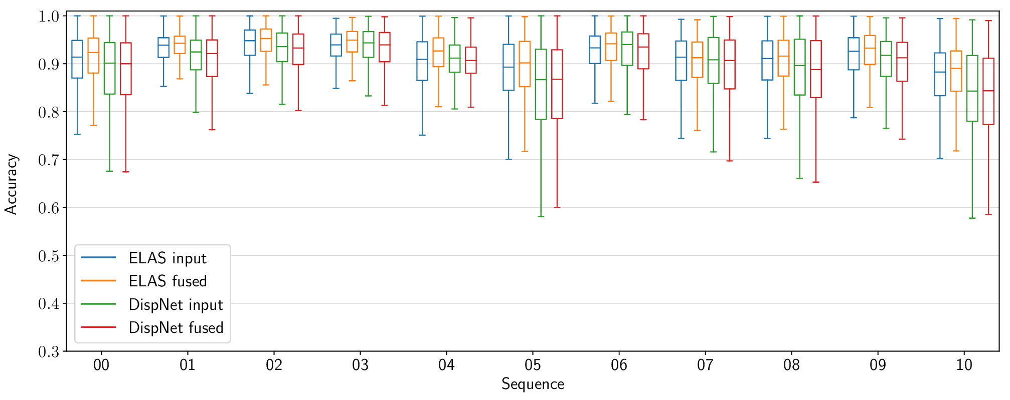
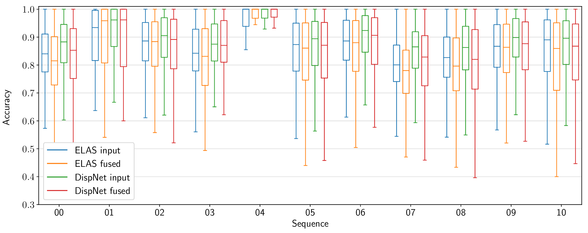
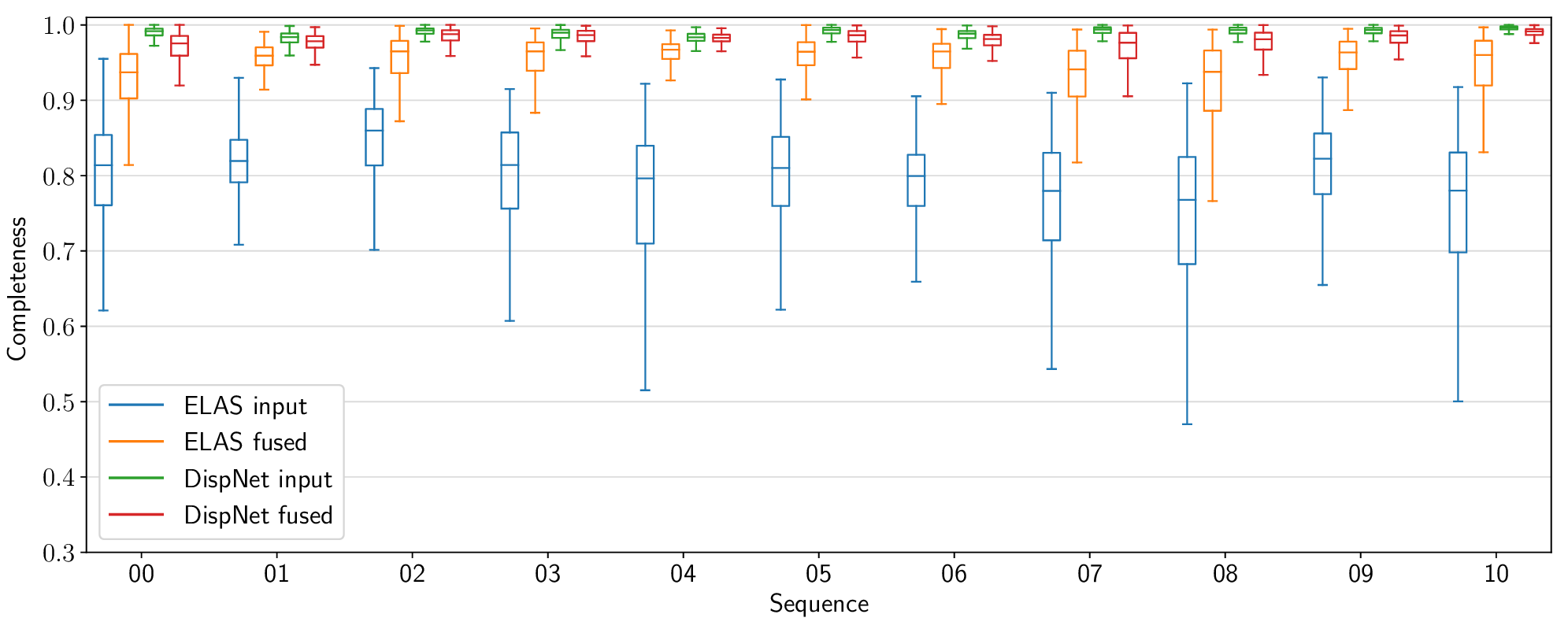
Reconstruction Accuracy
The following figures present per-sequence reconstruction accuracy results for the KITTI odometry dataset, as opposed to the aggregate results included in the paper.
Voxel Garbage Collection
Memory usage over time
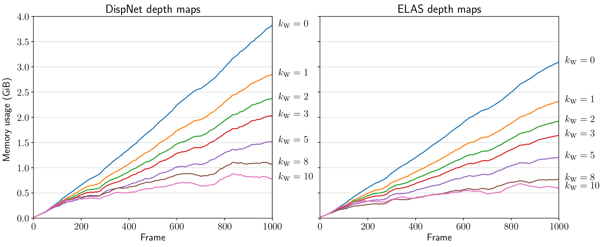
Fig 5. GPU memory usage over time for different regularization strengths \(k_\text{w}\). (Shorthand for \(k_\text{weight}\).) Experiment conducted on the first 1000 frames of KITTI odometry sequence 06.
Additional qualitative results
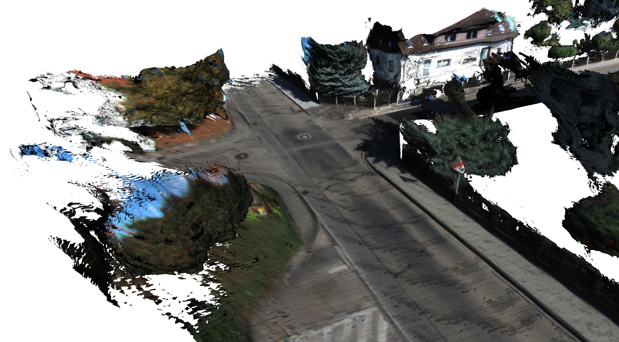
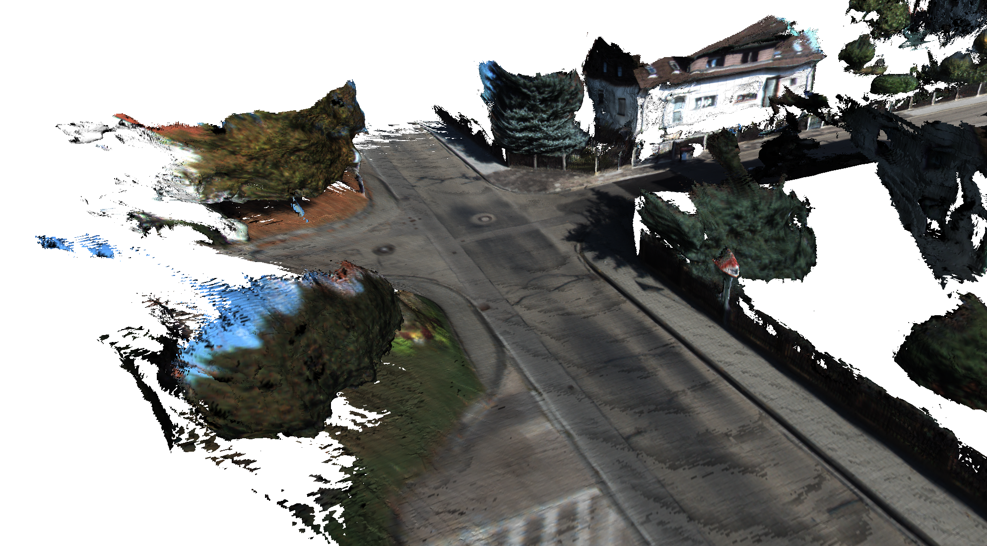
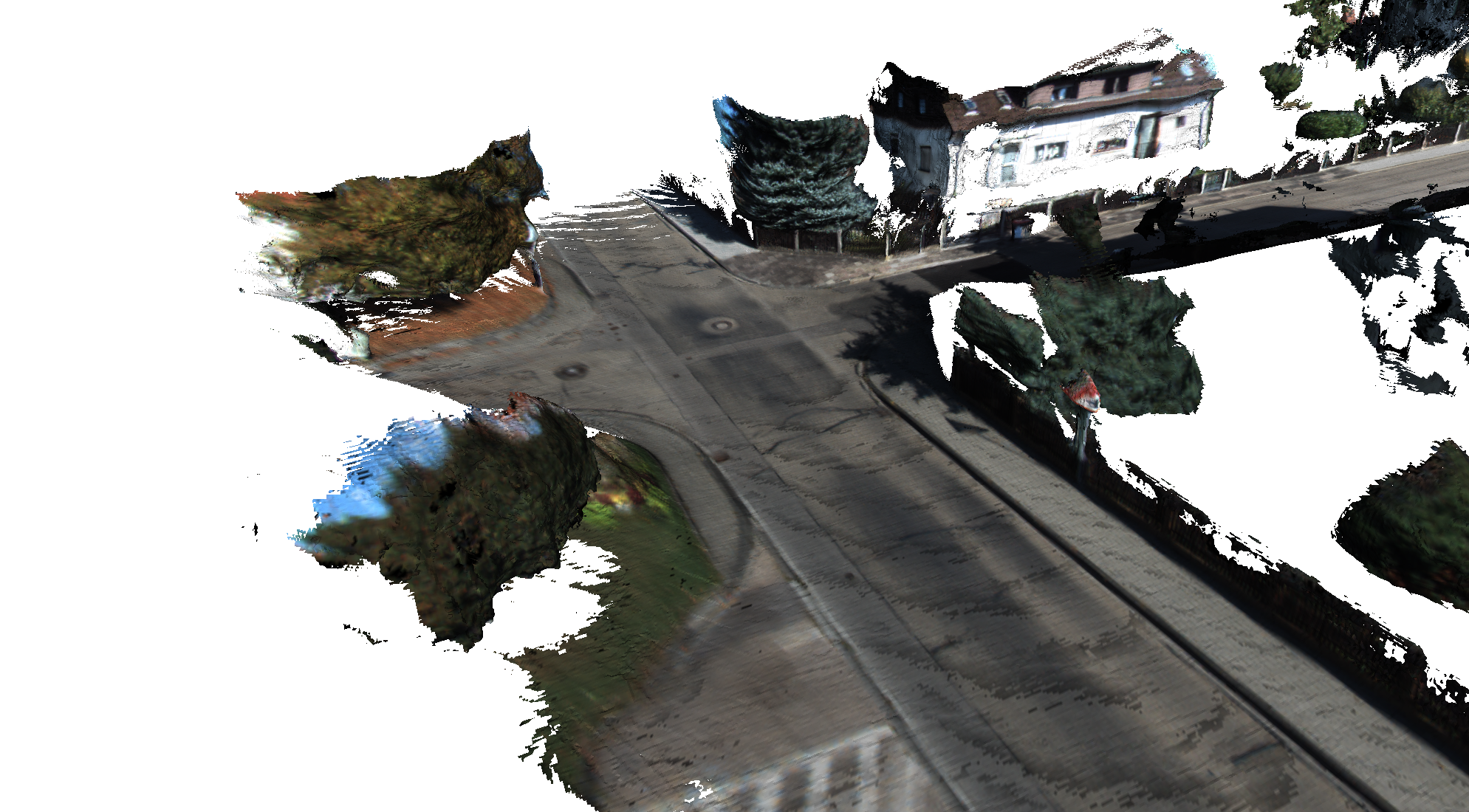
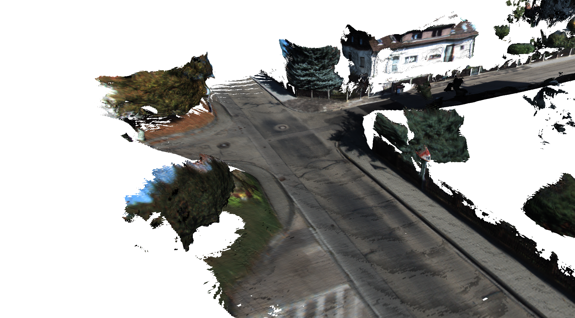
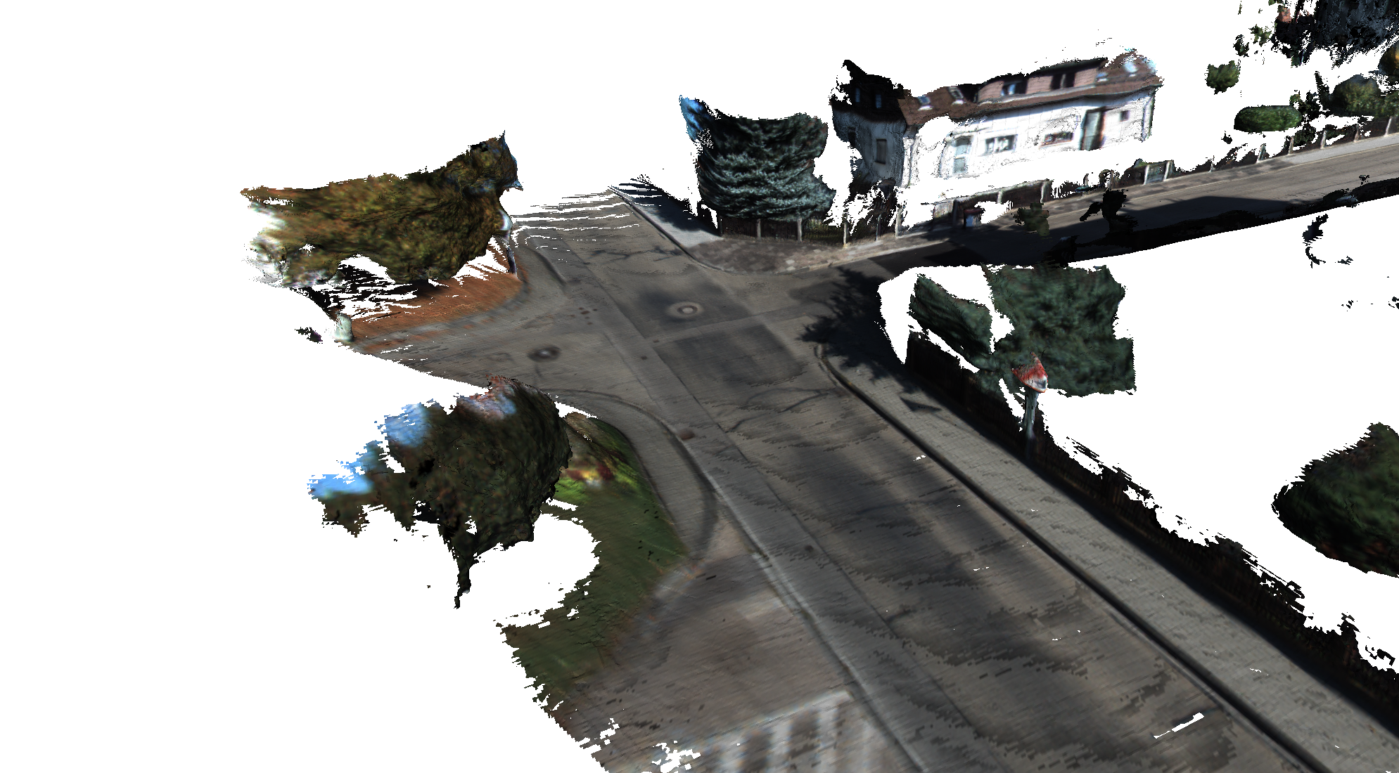
The reconstruction of an intersection under different regularization strengths can be seen below. Larger values of \(k_\text{weight}\) correspond to more aggressive noise thresholds.
Use the arrows to visualize values for different thresholds.
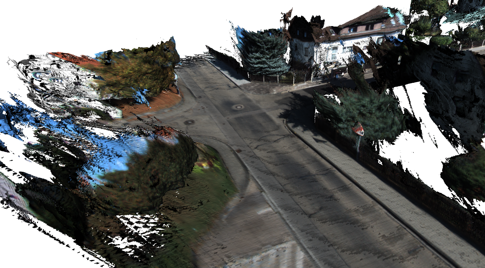
No voxel Garbage Collection
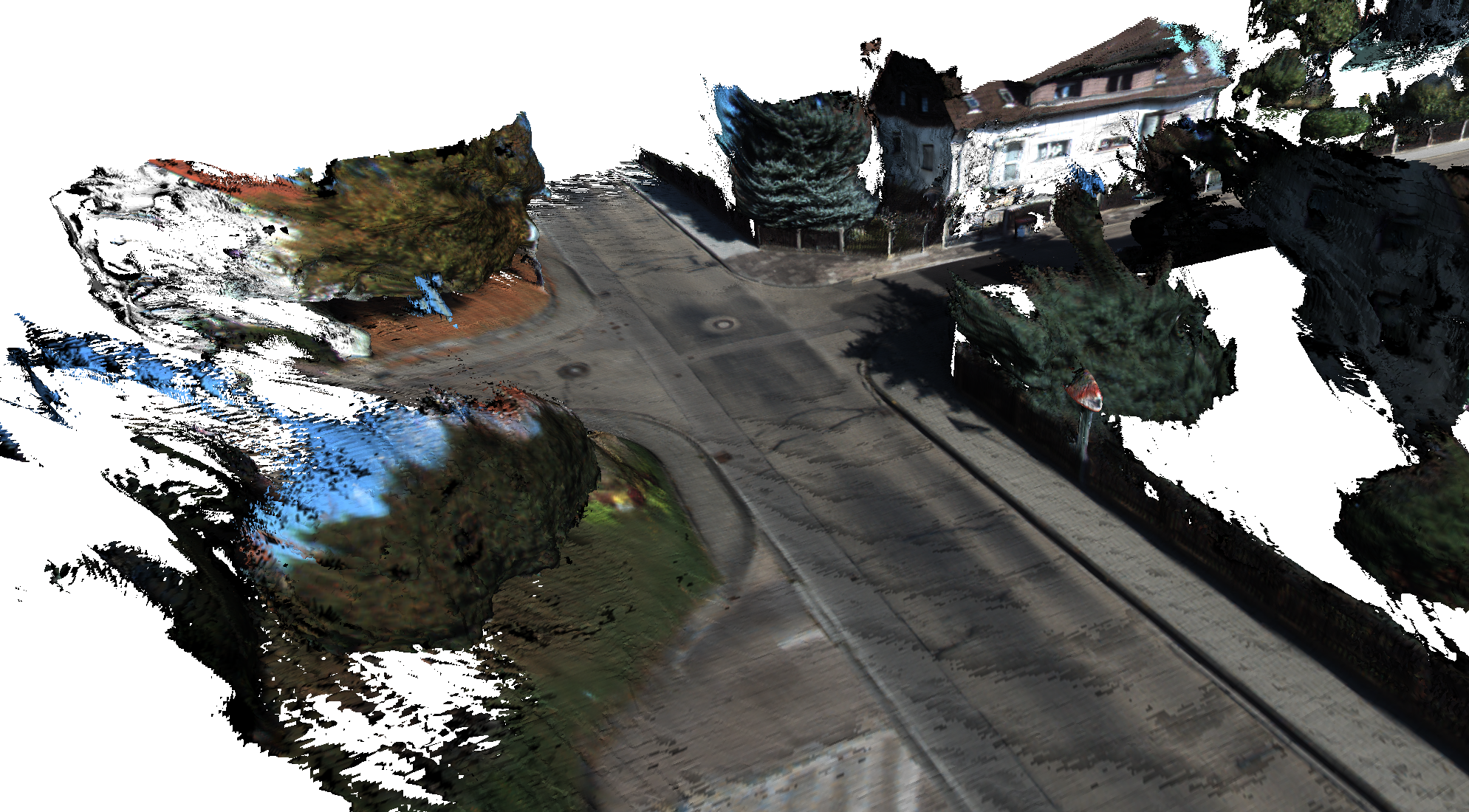
Voxel Garbage Collection with $$k_\text{weight}=1$$
Voxel Garbage Collection with $$k_\text{weight}=2$$
Voxel Garbage Collection with $$k_\text{weight}=3$$
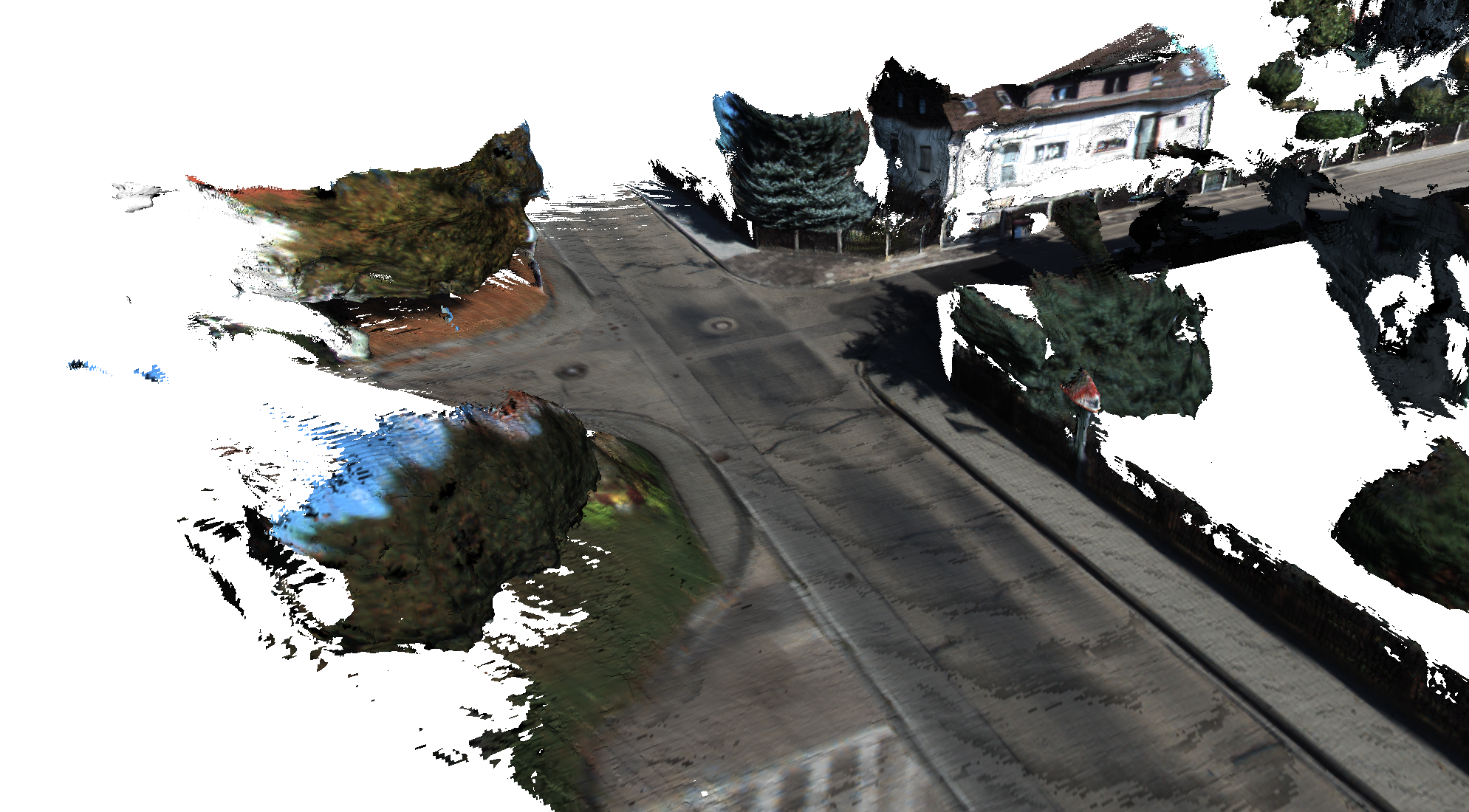
Voxel Garbage Collection with $$k_\text{weight}=4$$
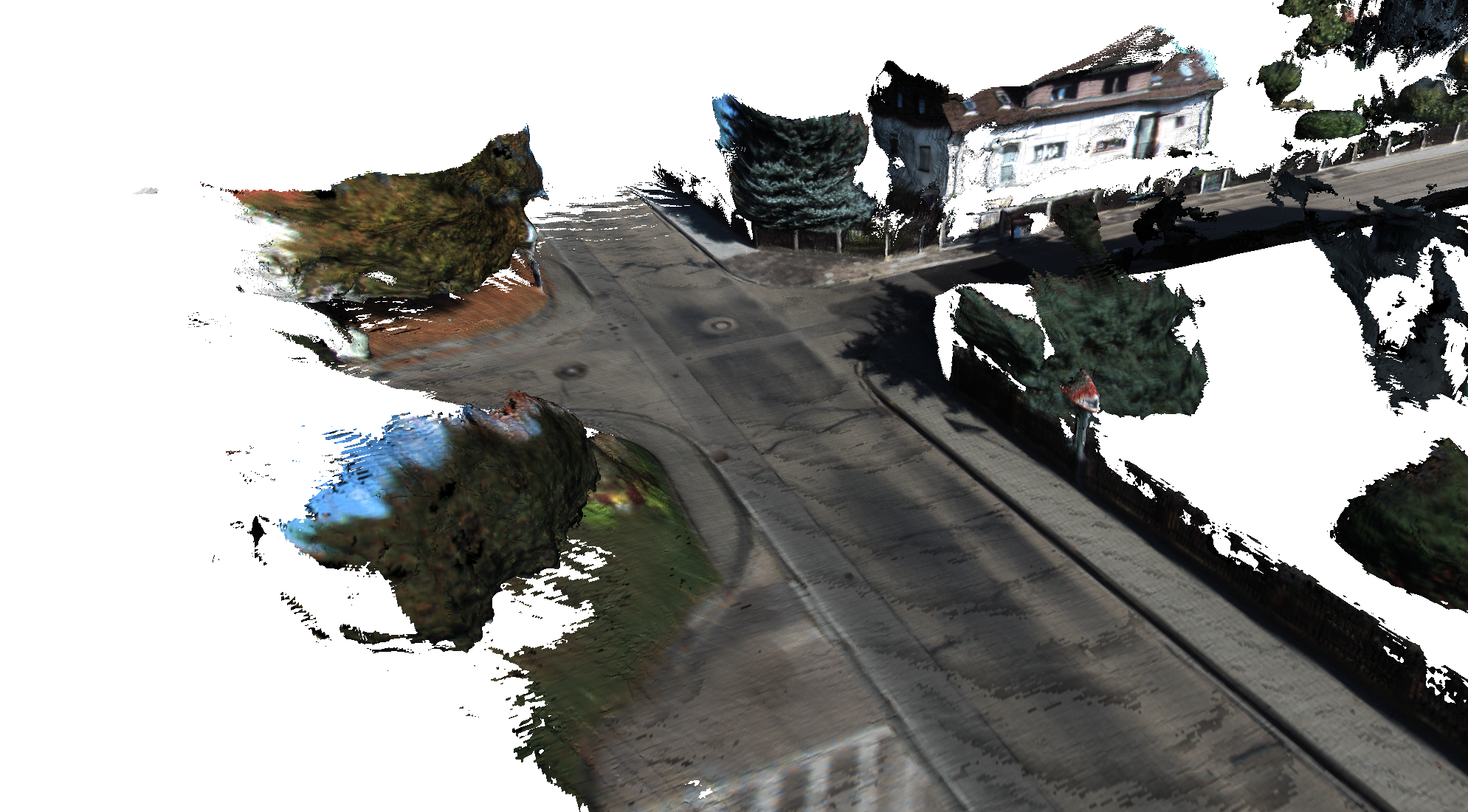
Voxel Garbage Collection with $$k_\text{weight}=5$$
Voxel Garbage Collection with $$k_\text{weight}=6$$
Voxel Garbage Collection with $$k_\text{weight}=7$$
Voxel Garbage Collection with $$k_\text{weight}=8$$
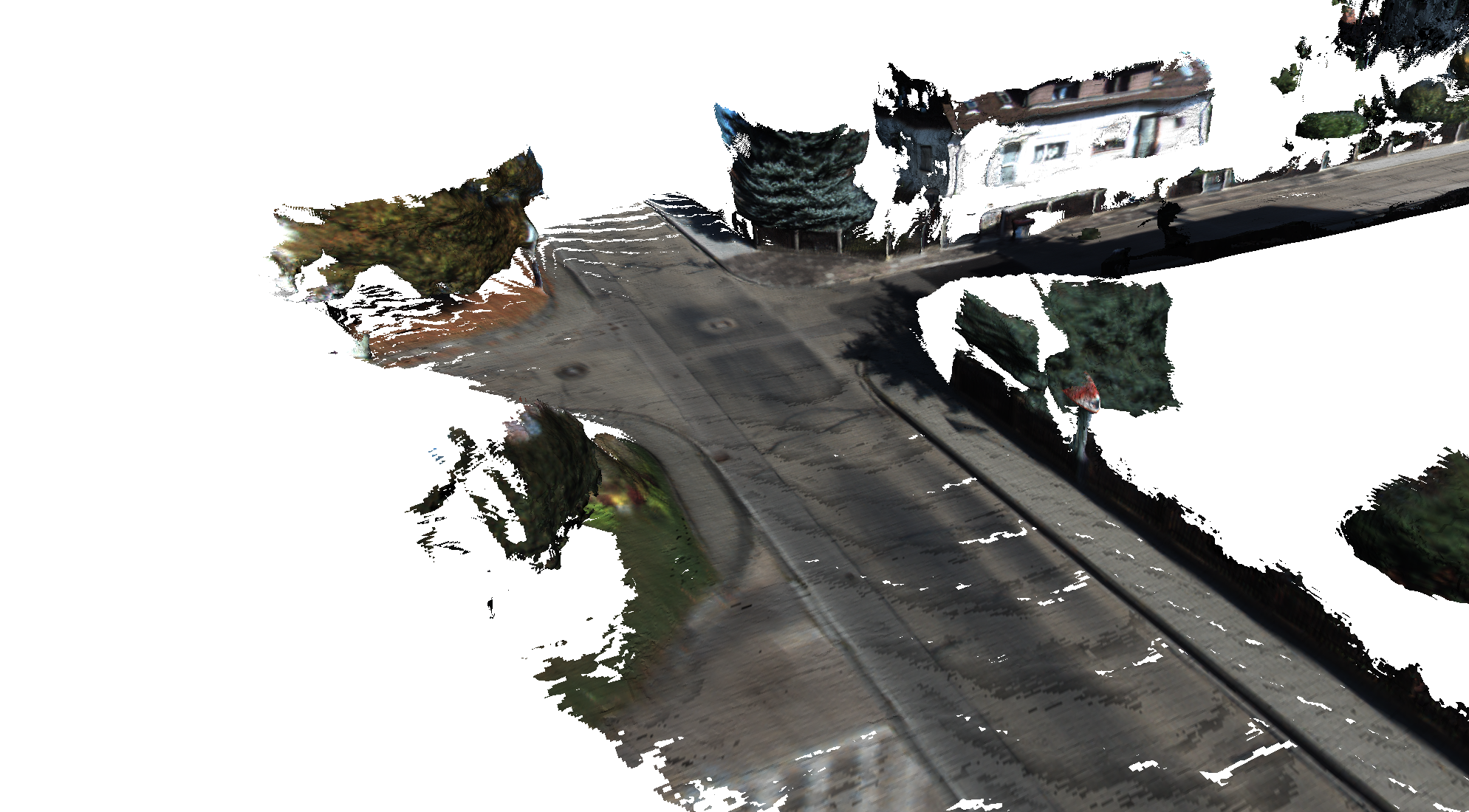
Voxel Garbage Collection with $$k_\text{weight}=10$$
Voxel Garbage Collection with $$k_\text{weight}=15$$
Voxel Garbage Collection with $$k_\text{weight}=20$$
Reduced Resolution Experiments
This section covers a series of experiments which investigated the impact of reducing the spatial and temporal resolution of the input on the reconstruction quality.
Reduced Input Spatial Resolution
We analyze the impact of the input spatial resolution on the accuracy and run time of DynSLAM. Most of these experiments are performed on KITTI odometry sequence number 6, which consists of 1101 frames exhibiting a good balance of buildings, vegetation, and traffic. Our findings reveal that, as would be expected, the reconstruction accuracy decreases with the input resolution. Similarly, the run time of some components, such as ELAS, also decreases when operating on lower-resolution input.
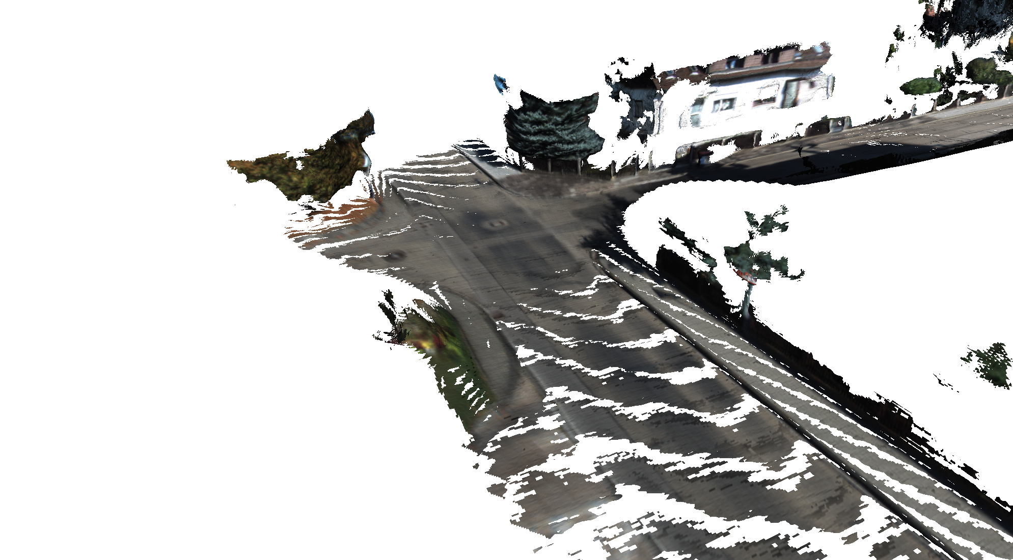
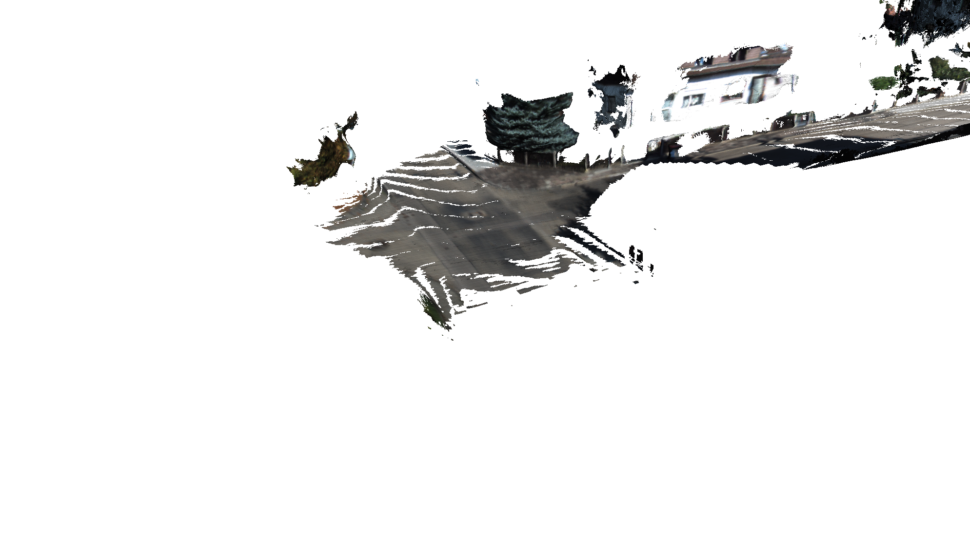
At the same time, we found that even when using 25% of the input dimensions, i.e., \(306 \times 92\) input, the system can still produce reasonable reconstructions, albeit only when using ELAS depth maps. The performance of DispNet drops significantly when using low-resolution input, leading to noisier reconstructions.
Table 1: Mean inference time for ELAS and MNC, the most time-consuming elements of our pipeline, as a function of the input resolution.
| Resolution | ELAS | MNC |
|---|---|---|
| 100% | 121ms (std=7ms) | 231ms (std=5ms) |
| 75% | 71ms (std=4ms) | 229ms (std=4ms) |
| 50% | 33ms (std=3ms) | 236ms (std=84ms) |
| 25% | 8ms (std=4ms) | 235ms (std=10ms) |
Table 1 shows the inference times of ELAS and the Multi-task Network Cascades, which are by far the most expensive operations in our system, as a function of the input resolution. Note that while the computation time of ELAS does decrease with the resolution of its inputs, the time taken by the instance-aware semantic segmentation does not. We conjecture that the reason behind this is the fixed number of object proposals (300, as mentioned in the original paper) generated by the first stage and refined by the second one. Despite lowering the input resolution, and with it, the cost of computing the convolutional image features, the run time of the pipeline ends up being bounded by the proposal generation, ranking, and refinement, which are almost completely independent of the input size in terms of their computational costs. Note that because of their generic nature, the processing times of the depth and instance-aware semantic segmentation components do not vary in significant ways across different KITTI sequences.
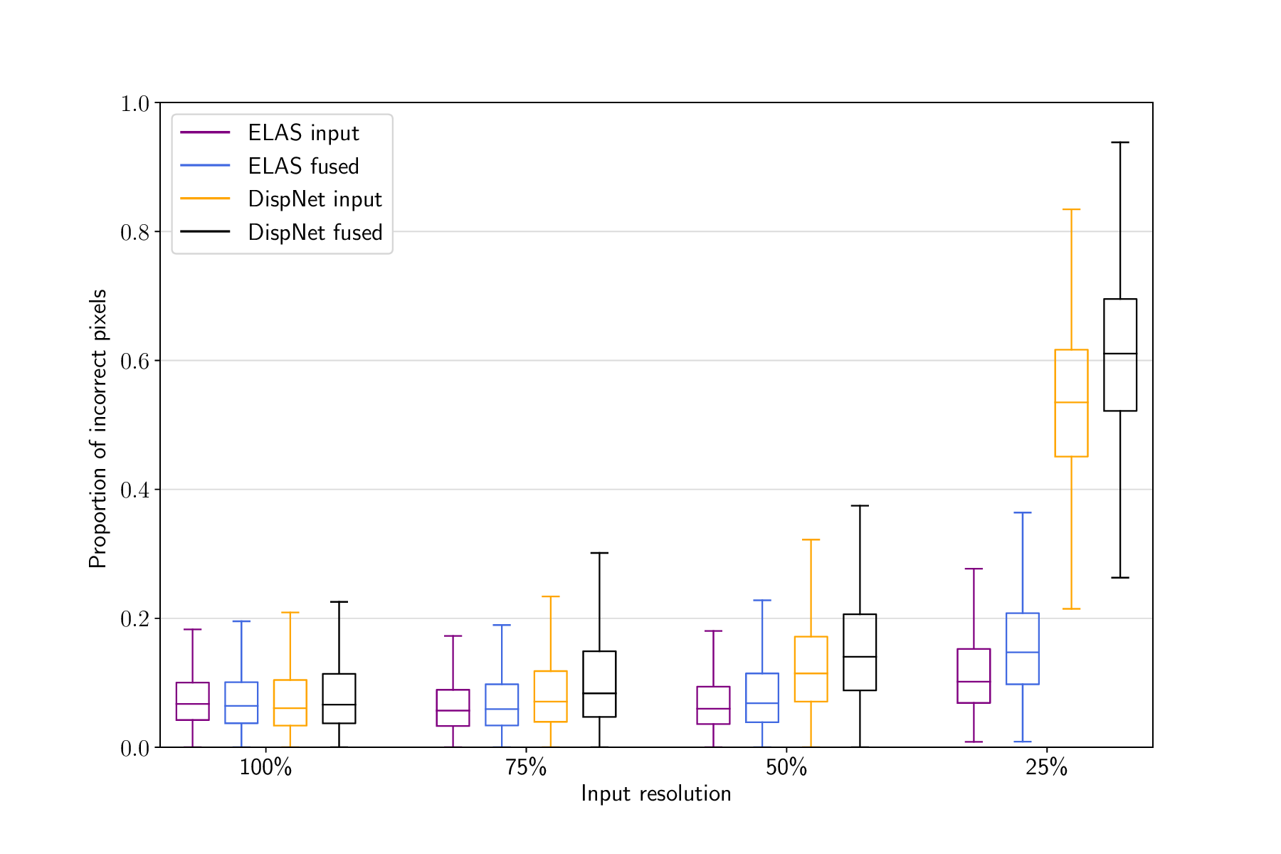 Figure 6: Input and reconstruction errors as functions of the input resolution.
The evaluation was performed on sequence 6 from the KITTI odometry benchmark.
Figure 6: Input and reconstruction errors as functions of the input resolution.
The evaluation was performed on sequence 6 from the KITTI odometry benchmark.
Figure 6 shows the reconstruction accuracy of DynSLAM as a function of the input resolution. As expected, the general trend is for the reconstruction error to increase as the resolution of the input is decreased. Nevertheless, for ELAS-based reconstruction, we notice a small increase in accuracy at 75%, as compared to 100% resolution. A possible explanation for this result is the fact that reducing the depth map resolution acts as a soft regularizer, reducing the impact of small bumps and other artifacts on the overall reconstruction quality. 75% resolution could therefore be seen as a “sweet spot” for good reconstructions, by reducing high-frequency noise associated with high-resolution depth maps, while at the same time having sufficient resolution to produce a faithful re- construction. Another interesting effect is the fact that as resolution decreases, the reconstruction (fused) error increases faster than the input error. This is due to the accumulation of errors in the map: if the depth maps become too degraded, artifacts begin to accumulate in the map, leading to errors over multiple sub- sequent frames. That is, an isolated erroneous (but large) bump in a depth map is registered as an input error only in the frame in which it is present. However, once it gets fused into the map, it might take several frames until subsequent measurements “smooth it out”. In other words, the regularizing effect of fusing depth maps across multiple frames can start to backfire when the quality of individual depth maps drops below a certain threshold, leading to severe map corruption caused by the cascading effects of artifacts from different input frames accumulating in the map. As is clearly visible in Figure 5.23, this effect is much more pronounced when using DispNet depth maps. This can be interpreted as a reflection of the fact that the DispNet architecture was only trained using high-resolution data. ELAS, not being reliant on training data, does not exhibit this problem, leading to reasonable results even at 306 × 92 resolution, i.e., less than QVGA.
In conclusion, we found that using ELAS to compute depth maps allows DynSLAM to function with acceptable accuracy even on very low-resolution input. On the other hand, while capable of producing qualitatively superior vehicle reconstructions on full-resolution input, DispNet depth maps lead to very poor performance on low-resolution (e.g., 25%) input.
Reduced Input Temporal Resolution
Given that the run time of our pipeline is dominated by the instance-aware semantic segmentation phase which, as seen in the previous subsection, takes roughly 250ms irrespective of the spatial resolution of the input, we present a series of preliminary experiments investigating the possibility of avoiding to run the computationally expensive segmentation every frame. In other words, we consider the option of running cheaper components such as visual odometry on every input frame, but only computing dense depth maps, the instance-aware semantic segmentation, and the static map fusion every k frames, with the hope that it would allow the system to operate closer to real time, without significant losses in terms of mapping accuracy and completeness. Early experiments showed that the 3D object tracking performs rather poorly even when it is run every two frames instead of every frame, but that the static map fusion remains accurate even when performed every 3–5 frames. Because of this behavior, we choose to focus on evaluating the quality of the dense depth map, using the non-semantic (i.e., full-frame) method described in the paper. As such, we use the first 1000 frames of KITTI odometry sequence 09, which contain almost no dynamic objects.
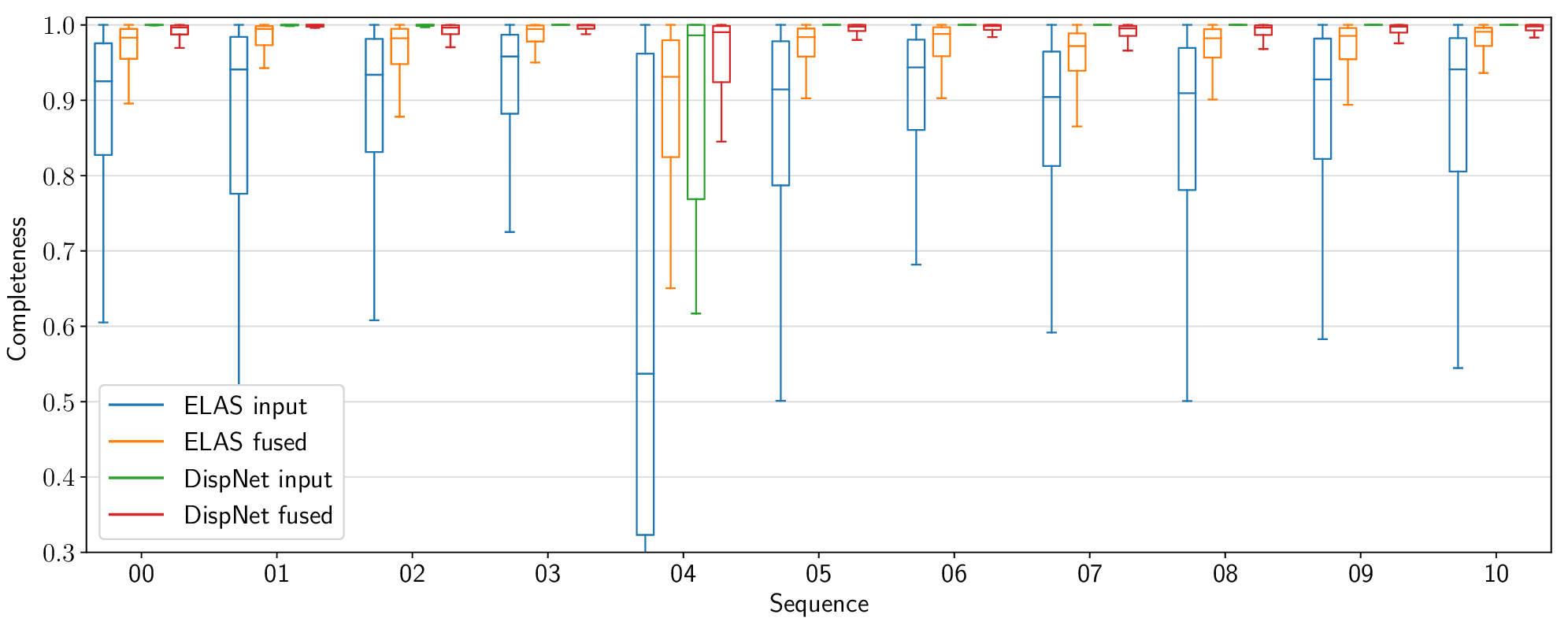
The results of this experiment are shown in Figures 7 and 8. As expected, on its own, the accuracy of the reconstruction is not affected since the input depth maps are themselves accurate. On the other hand, the reconstruction completeness score starts to drop significantly once fusion is performed more rarely than every 4–5 frames. In conclusion, the high completeness and accuracy scores obtained even when performing the static map fusion every two or three frames show that it is not necessary to perform this operation at input frequency. In the future, this insight could be used to improve the efficiency of similar systems, prioritizing tasks such as object tracking and planning to run on every frame, but performing auxiliary tasks such as mapping with a lower frequency.
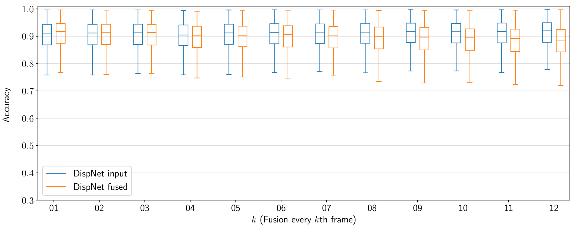 Figure 7: The impact of reduced temporal resolution on static map reconstruction
accuracy. A value of k = 1 signifies fusion performed every
frame (the default case), k = 2, every two frames, etc.
Figure 7: The impact of reduced temporal resolution on static map reconstruction
accuracy. A value of k = 1 signifies fusion performed every
frame (the default case), k = 2, every two frames, etc.
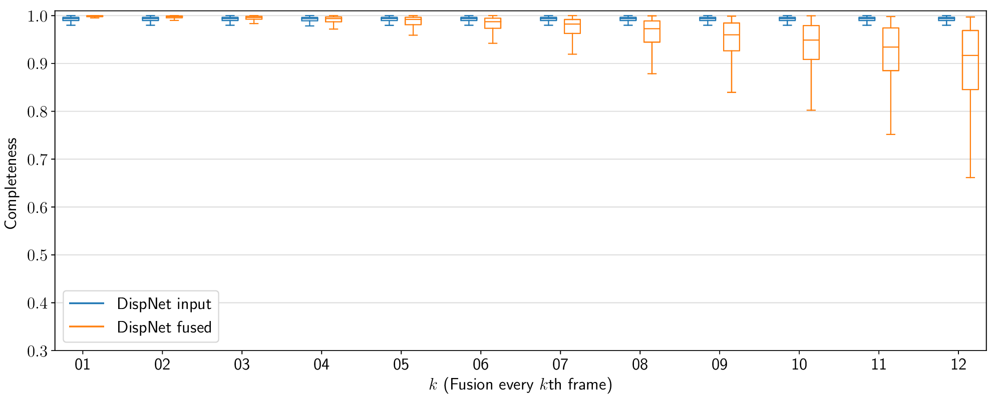 Figure 8: The impact of reduced temporal resolution on static map reconstruction
accuracy.
Figure 8: The impact of reduced temporal resolution on static map reconstruction
accuracy.
BibTeX
@inproceedings{Barsan2018ICRA,
    title = {Robust Dense Mapping for Large-Scale Dynamic Environments},
    author = {B{\^a}rsan, Ioan Andrei and Liu, Peidong and Pollefeys, Marc and
              Geiger, Andreas},
    booktitle = {Proceedings of the IEEE International Conference on Robotics
                 and Automation ({ICRA}) 2018},
    publisher = ,
    month = may,
    year = {2018},
    month_numeric = {5}
}